3.1 Total Score & Difficulty
Item difficulty \(p_i\) is defined as probability of test takers answering the item \(i\) correct. This is estimated by \(p_i = \frac{\text{# of test takers who answered correctly}}{\text{total # of test takers}}\). Let’s take a look at the relationship between \(p_i\) and total score (sum of number of items correct, equally-weighted). In the following simulation, 15-item tests are administered to 1000 people. Different tests have different levels of difficulties for the underlying items.
Code to simulate tests taken
# For a test with "item_n" number of items,
#   generate a dataset where "person_n" number of people answered the 15 items.
# For all people, each item has "prob" probability of answering correctly.
#   The vector of "prob" recycles to all the items.
#   For example,
#    "prob = 0.5" means all items have 50% chance of correct
#    "prob = c(0.25, 0.75)" means item 1 has 25% chance, item 2 has 75% chance,
#                                 item 3 has 25% chance, item 4 has 75% chance,
#                                 ... until you run out of item
make_test_score_df <- function(item_n, person_n, prob = 0.5) {
  if (length(prob) == 1) {
    df <- sapply(seq_len(item_n), function(i) { rbinom(person_n, size = 1, prob = prob) })
  } else {
    # if prob for all items not specified, recycle to the length of item_n
    prob <- rep_len(prob, item_n)
    res <- lapply(seq_along(prob), function(i) {
      rbinom(person_n, size = 1, prob[i])
    })
    df <- matrix(unlist(res), ncol = item_n, nrow = person_n, byrow = F)
  }

  colnames(df) <- paste0(rep("Item ", item_n), seq_len(item_n))

  df <- df %>% as_tibble() %>%
    mutate(Person =  paste0(rep("Person ", person_n), seq_len(person_n))) %>%
    pivot_longer(cols = 1:15, names_to = "Item")

  df
}

# Create Density Plot for simulated dataset
make_test_score_plot <- function(df, item_n, person_n, subtitle = "") {
  df_Score_by_Person <- df %>%
    group_by(Person) %>%
    summarise(
      Score = sum(value)
    )
  as_tibble(
    df_freq <- as.data.frame.table(
      table(Score = factor(df_Score_by_Person$Score, levels = seq(0, item_n, by = 1))),
      responseName='Frequency'))
  df_freq %>%
    mutate(RelativeFrequency = Frequency/person_n,
           Score = as.numeric(as.character(Score))) %>%
    ggplot(aes(x = Score, y = RelativeFrequency)) +
    geom_point() + geom_line() +
    scale_x_continuous(name = "Score",
                       breaks = seq(0, item_n, by = 1),
                       minor_breaks = seq(0, item_n, by = 1),
                       limits = c(0, item_n)) +
    stat_function(fun = dnorm,
                  args = list(mean = item_n * 0.5, sd = item_n * 0.5 * (1-0.5)), # expected normal distribution at p = 0.5
                  col = "red") +
    ggtitle(label = paste0("Distribution of Test Scores for ", person_n, " test takers."),
            subtitle = subtitle) +
    ylab("Relative Frequency")
}
Now we generate 15-item test administered to 1000 people and plot the total score against theoretically normally distributed total score. Note the diffculty \(p_i\) (prob in the R code)
df_p25 <- make_test_score_df(item_n = 15, person_n = 1000, prob = 0.25)
make_test_score_plot(df_p25, item_n = 15, person_n = 1000, subtitle = (expression(paste("All items: ", p[i], " = ", 0.25," (hard)"))))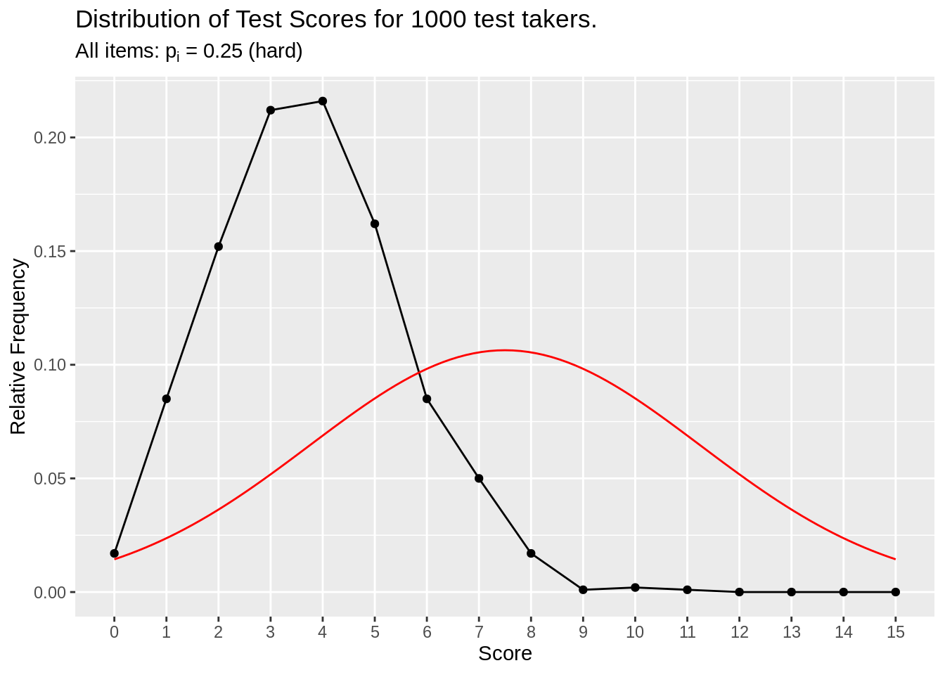
Figure 3.1: All hard item simulation
Items have hard difficulty (25% chance of correct), so the total score for test takers are right skewed.
df_p50 <- make_test_score_df(item_n = 15, person_n = 1000, prob = 0.50)
make_test_score_plot(df_p50, item_n = 15, person_n = 1000, subtitle = (expression(paste("All items: ", p[i], " = ", 0.50," (medium)"))))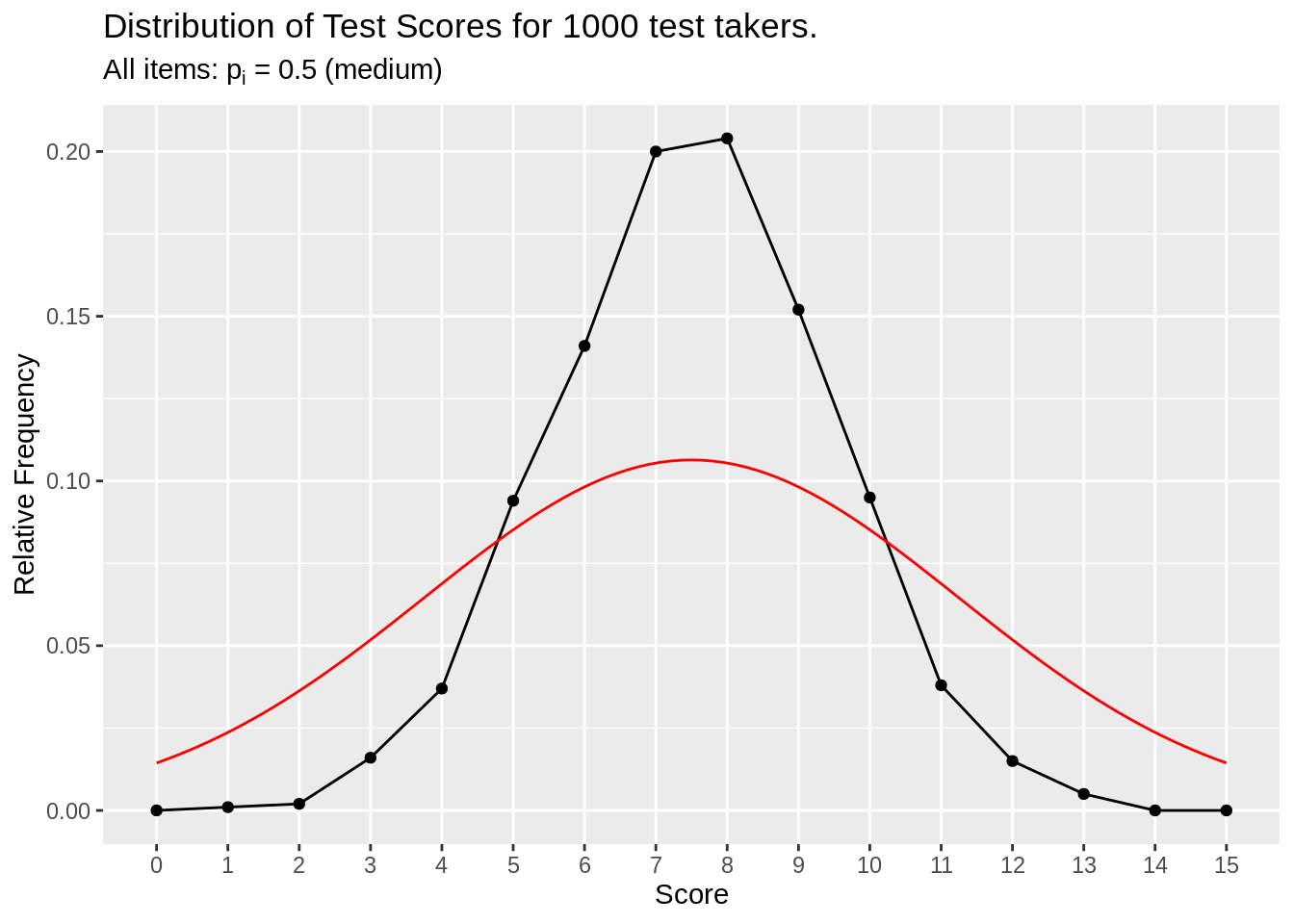
Figure 3.2: All medium item simulation
Items have medium difficulty (50% chance of correct), so the total score for test takers are normally distributed.
TODO compare kurtosis?
df_p75 <- make_test_score_df(item_n = 15, person_n = 1000, prob = 0.75)
make_test_score_plot(df_p75, item_n = 15, person_n = 1000, subtitle = (expression(paste("All items: ", p[i], " = ", 0.75," (easy)"))))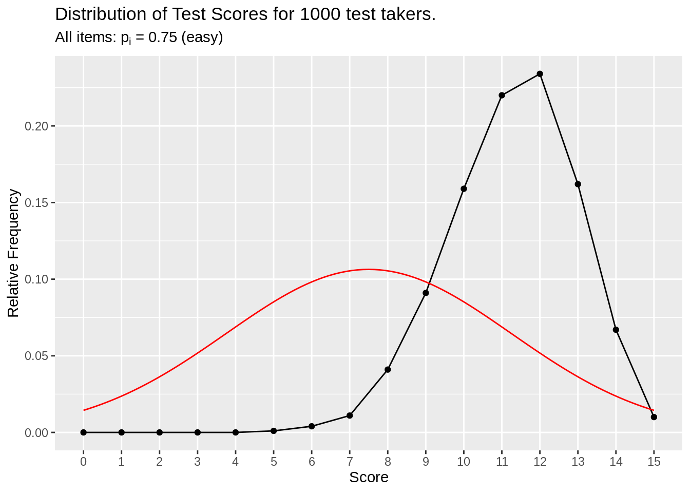
Figure 3.3: All easy item simulation
Items have east difficulty (75% chance of correct), so the total score for test takers are left skewed.
df_p02 <- make_test_score_df(item_n = 15, person_n = 1000, prob = 0.02)
make_test_score_plot(df_p02, item_n = 15, person_n = 1000, subtitle = (expression(paste("All items: ", p[i], " = ", 0.02," (very hard)"))))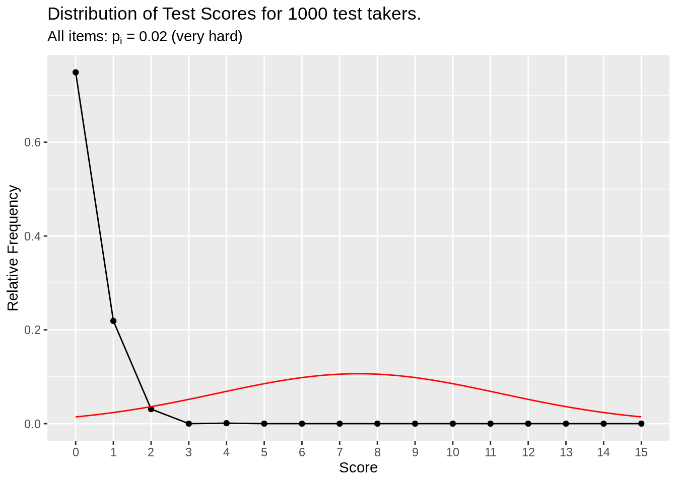
Figure 3.4: All very hard item simulation
Items have very hard difficulty (2% chance of correct), so the total score for test takers are highly right skewed. This test isn’t useful (Other than maybe identifying that one-in-a-million genius. Regardless, this test is not discriminatory).
df_p98 <- make_test_score_df(item_n = 15, person_n = 1000, prob = 0.98)
make_test_score_plot(df_p98, item_n = 15, person_n = 1000, subtitle = (expression(paste("All items: ", p[i], " = ", 0.98," (very easy)"))))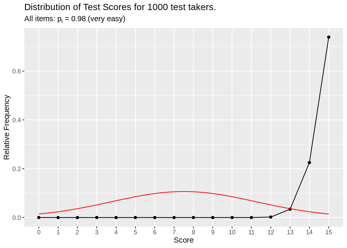
Figure 3.5: All very easy item simulation
Items have very easy difficulty (98% chance of correct), so the total score for test takers are highly left skewed. This test isn’t useful because everyone will get perfect or near perfect scores.
So what is an ideal test? A good mixture of items varying diffculty around 0.30 - 0.70 (for average of 0.5).
But if we are targeting ~0.50 for all items taken together, why not alternate between very hard (\(p_i = 0.02\)) and very easy (\(p_i = 0.98\)) for the ~0.50? Wouldn’t that lead to the same thing?
# Leptokurtic distribution of test scores bc items are too hard or too easy
df_p02_p98 <- make_test_score_df(item_n = 15, person_n = 1000, prob = c(0.02, 0.98))
make_test_score_plot(df_p02_p98, item_n = 15, person_n = 1000,
                     subtitle = (expression(paste("All items: ", p[i]," = 0.02 or ", p[i], ", = 0.98 (very hard or very easy)"))))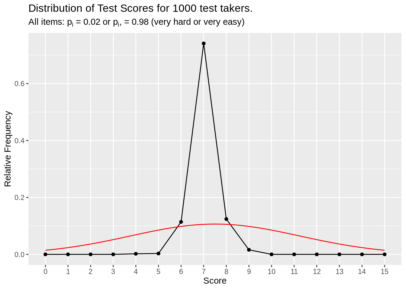
Figure 3.6: Very hard or very easy item simulation
The simulation shows that the total score distribution is piling up in the middle, creating highly leptokurtic distribution. To fix this, you have to add more MEDIUM LEVEL items to distribute item’s contribution to the total score to both ends of the total score
# To fix, add more moderate difficutly tests
df_p02_p50_p98 <- make_test_score_df(item_n = 15, person_n = 1000, prob = c(0.02 , 0.50, 0.50, 0.50, 0.98))
make_test_score_plot(df_p02_p50_p98, item_n = 15, person_n = 1000,
                     subtitle = (expression(paste("All items: ", p[i]," = {0.02 , 0.50, 0.50, 0.50, 0.98}"))))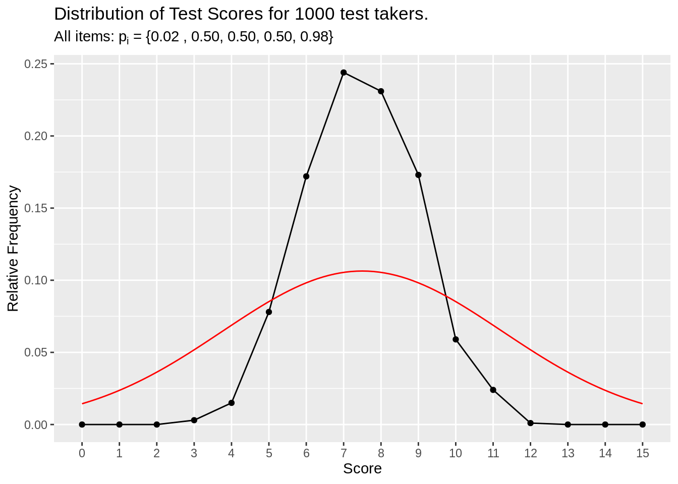
Figure 3.7: Medium difficulty added item simulation
At first, you might think “If too many people are scoring ~7.5 (50% of possible max 15), then why should the items be medium diffculty such that 50% of the test takers would answer correctly? Shouldn’t I add more easy / hard items?” Well in the simulation example 3.6, we took “add more easy / hard items” to the extreme where all items were only very easy or very hard. This distribution happens because score is the total sum of individual item’s correct (1) or incorrect (0). If half of the items were very hard, the sum of those very hard items would be 0 or near 0. On the other hand, the other half of very easy items would have sum of 7 or nearly 8 (or ~8, because we have odd number of items). When you add these halves togehter, the total score hovers around the middle score of ~7.5.